38 excel pie chart add labels

spreadsheetplanet.com › bar-of-pie-chart-excelHow to Create Bar of Pie Chart in Excel? Step-by-Step Excel lets us add our own customizations to the Bar of Pie chart. For example, it lets us specify how we want the portions to get split between the pie and the stacked bar. It also lets us specify whether we want to display data labels, what data labels we want to be displayed as well as what formatting and styling we want to apply to the labels. › documents › excelHow to display leader lines in pie chart in Excel? To display leader lines in pie chart, you just need to check an option then drag the labels out. 1. Click at the chart, and right click to select Format Data Labels from context menu. 2. In the popping Format Data Labels dialog/pane, check Show Leader Lines in the Label Options section. See screenshot: 3. Close the dialog, now you can see some leader lines appear. If you want to show all leader lines, just drag the labels out of the pie one by one.

excel - How to not display labels in pie chart that are 0% - Stack Overflow Generate a new column with the following formula: =IF (B2=0,"",A2) Then right click on the labels and choose "Format Data Labels". Check "Value From Cells", choosing the column with the formula and percentage of the Label Options. Under Label Options -> Number -> Category, choose "Custom". Under Format Code, enter the following:

Excel pie chart add labels

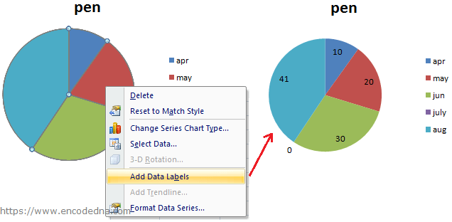
Add a DATA LABEL to ONE POINT on a chart in Excel All the data points will be highlighted. Click again on the single point that you want to add a data label to. Right-click and select ' Add data label '. This is the key step! Right-click again on the data point itself (not the label) and select ' Format data label '. You can now configure the label as required — select the content of ... › 2018/09/12 › add-line-excel-graphHow to add a line in Excel graph (average line, benchmark ... Sep 12, 2018 · To achieve this effect, add a line to your chart as explained in the previous examples, and then do the following customizations: In your graph, double-click the target line. This will select the line and open the Format Data Series pane on the right side of your Excel window. c# - Add data labels to excel pie chart - Stack Overflow Add data labels to excel pie chart. Bookmark this question. Show activity on this post. private void DrawFractionChart (Excel.Worksheet activeSheet, Excel.ChartObjects xlCharts, Excel.Range xRange, Excel.Range yRange) { Excel.ChartObject myChart = (Excel.ChartObject)xlCharts.Add (200, 500, 200, 100); Excel.Chart chartPage = myChart.Chart;

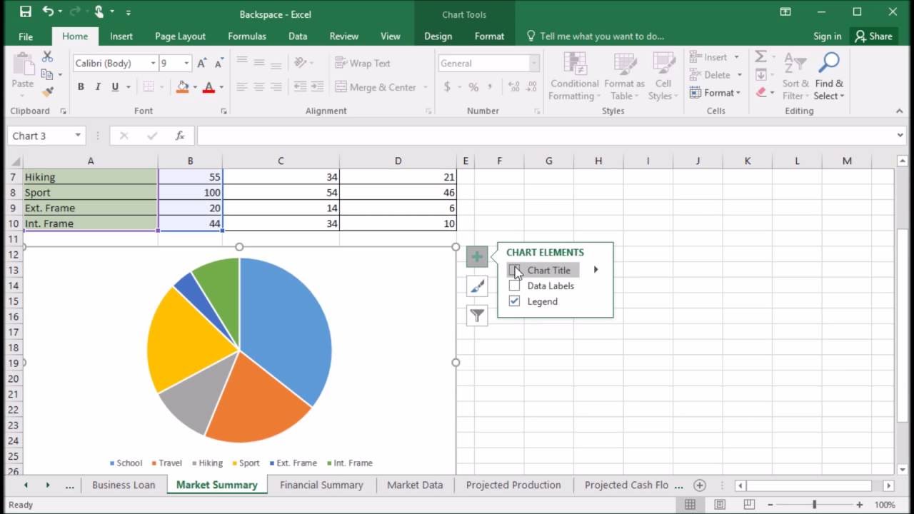
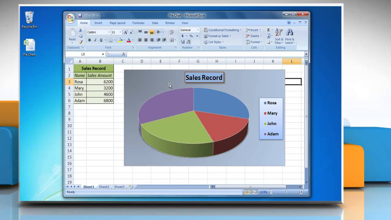
Excel pie chart add labels. Pie Chart in Excel - Inserting, Formatting, Filters, Data Labels To add Data Labels, Click on the + icon on the top right corner of the chart and mark the data label checkbox. You can also unmark the legends as we will add legend keys in the data labels. We can also format these data labels to show both percentage contribution and legend:- Right click on the Data Labels on the chart. › legends-in-chartHow To Add and Remove Legends In Excel Chart? - EDUCBA This has been a guide to Legend in Chart. Here we discuss how to add, remove and change the position of legends in an Excel chart, along with practical examples and a downloadable excel template. You can also go through our other suggested articles – Line Chart in Excel; Excel Bar Chart; Pie Chart in Excel; Scatter Chart in Excel Creating Pie Chart and Adding/Formatting Data Labels (Excel) Creating Pie Chart and Adding/Formatting Data Labels (Excel) - YouTube. › combo-chart-in-excelHow to Create Combo Chart in Excel? - EDUCBA Step 9 – Add the Chart Title as “Combination Chart” under the Chart Title section under combo graph. You can use more customizations like changing the design of the graph, adding axis labels or changing series bars and series line colors, changing widths, etc., to make your graph visually more pleasant.

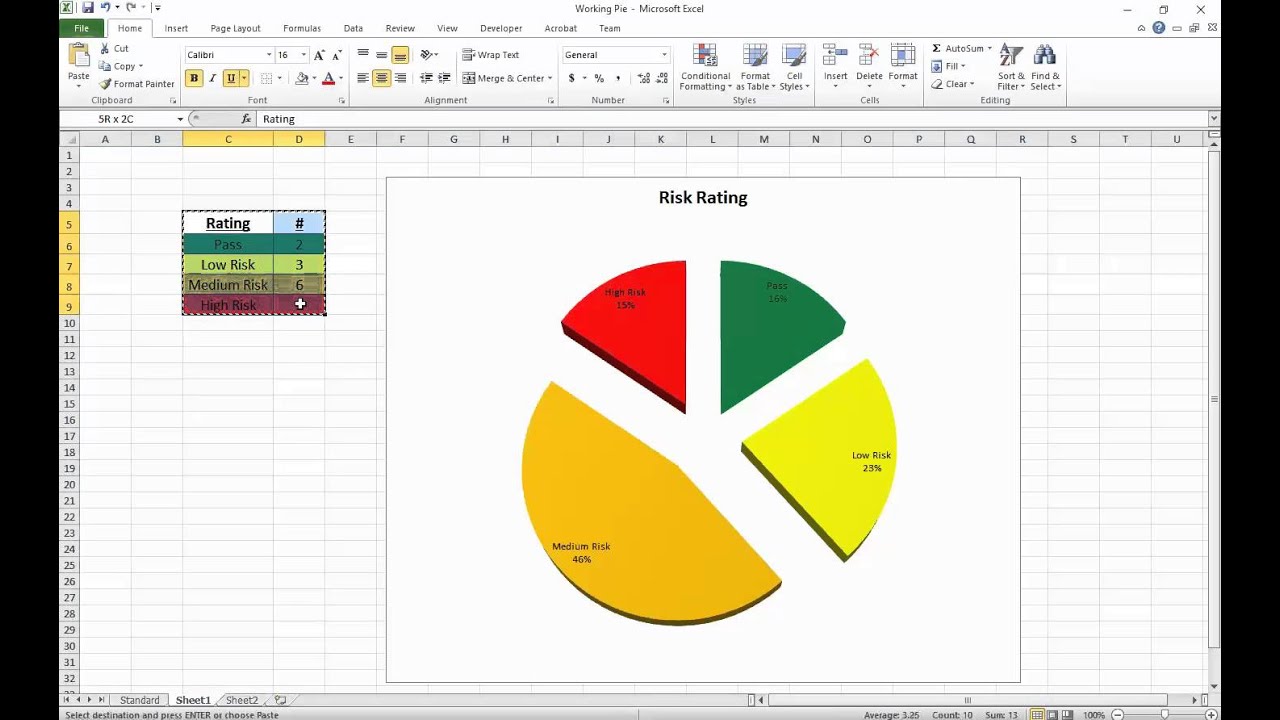
Inserting Data Label in the Color Legend of a pie chart Re: Inserting Data Label in the Color Legend of a pie chart @SabrinaFr There is no built-in way to do that, but you can use a trick: see Add Percent Values in Pie Chart Legend (Excel 2010) Adding data labels to a Pie Chart in VBA - Automate Excel Adding data labels to a Pie Chart in VBA - Automate Excel. support.microsoft.com › en-us › officeAdd a pie chart - support.microsoft.com To switch to one of these pie charts, click the chart, and then on the Chart Tools Design tab, click Change Chart Type. When the Change Chart Type gallery opens, pick the one you want. See Also. Select data for a chart in Excel. Create a chart in Excel. Add a chart to your document in Word. Add a chart to your PowerPoint presentation Excel Show Percentage Pie Chart - TheRescipes.info Please do as follows to create a pie chart and show percentage in the pie slices. 1. Select the data you will create a pie chart based on, click Insert > I nsert Pie or Doughnut Chart > Pie. See screenshot: 2. Then a pie chart is created. Right click the pie chart and select Add Data Labels from the context menu. 3.

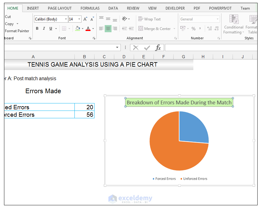
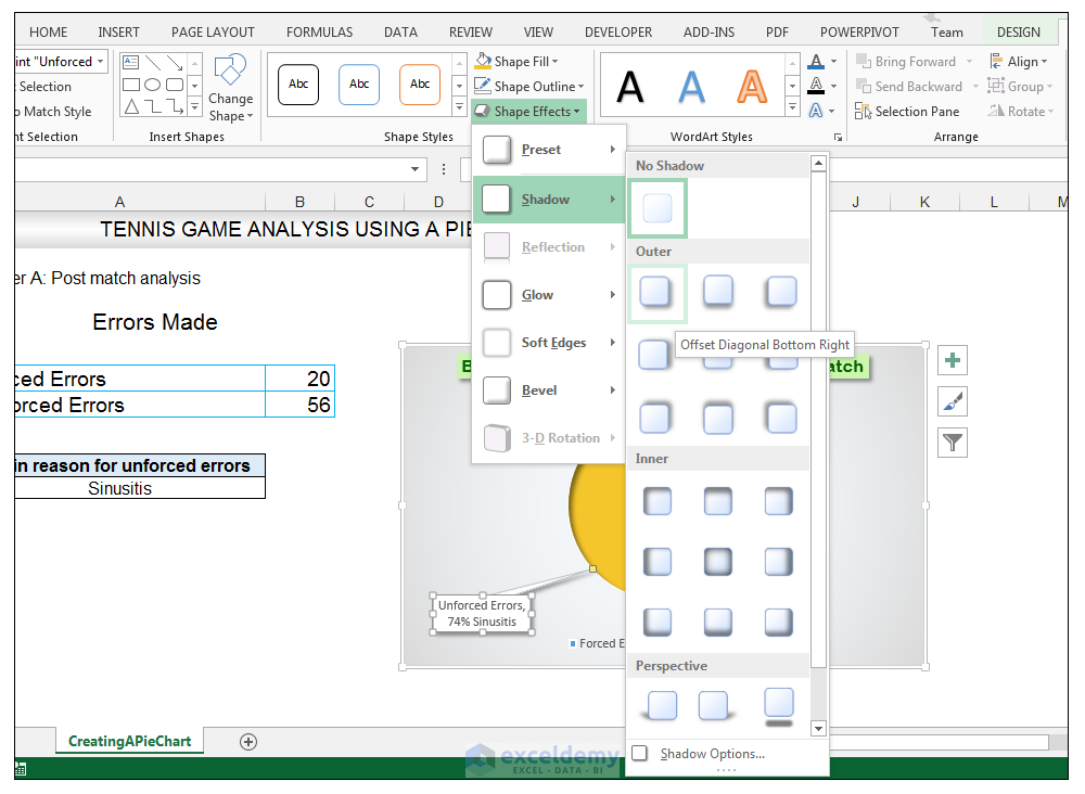
How to Make a Pie Chart in Excel & Add Rich Data Labels to The Chart! Creating and formatting the Pie Chart. 1) Select the data. 2) Go to Insert> Charts> click on the drop-down arrow next to Pie Chart and under 2-D Pie, select the Pie Chart, shown below. 3) Chang the chart title to Breakdown of Errors Made During the Match, by clicking on it and typing the new title. 4) With the chart title still selected, go to ... How to Create and Format a Pie Chart in Excel - Lifewire To add data labels to a pie chart: Select the plot area of the pie chart. Right-click the chart. Select Add Data Labels . Select Add Data Labels. In this example, the sales for each cookie is added to the slices of the pie chart. › solutions › excel-chatHow To Add a Title To A Chart or Graph In Excel – Excelchat We will go the Design tab, then Add Chart Element, Tap Chart Title and pick More Title options. Here we will be able to change color, font style, etc. **In Excel 2010, we go to Labels, Layout Tab and then Chart Title in the More Title Options. We can quickly Right-click on the Chart Title Box and select Format Chart Title; Figure 5 ... Microsoft Excel Tutorials: Add Data Labels to a Pie Chart To add the numbers from our E column (the viewing figures), left click on the pie chart itself to select it: The chart is selected when you can see all those blue circles surrounding it. Now right click the chart. You should get the following menu: From the menu, select Add Data Labels. New data labels will then appear on your chart:

How to Make a Pie Chart in Excel & Add Rich Data Labels to The Chart!

Where are data labels in Excel? - Foley for Senate To format data labels in Excel, choose the set of data labels to format. To do this, click the "Format" tab within the "Chart Tools" contextual tab in the Ribbon. Then select the data labels to format from the "Chart Elements" drop-down in the "Current Selection" button group.

406 How to remove chart title and add data labels to a Pie Chart in Excel 2016 - YouTube

Office: Display Data Labels in a Pie Chart - Tech-Recipes 3. In the Chart window, choose the Pie chart option from the list on the left. Next, choose the type of pie chart you want on the right side. 4. Once the chart is inserted into the document, you will notice that there are no data labels. To fix this problem, select the chart, click the plus button near the chart's bounding box on the right ...

Change the colours of a Pie Chart to represent the data FIgures using VBA - YouTube

ΜΑΘΗΜΑ 1 - fernio Άνοιγμα Της Εφαρμογής Υπολογιστικών Φύλλων (Microsoft Excel) ... Αλλάξετε τον τύπο του γραφήματος/chart type σε γράφημα πίτας 2Δ/2D pie.72 σελίδες

VBA Guide For Charts and Graphs - Automate Excel

How to Insert Axis Labels In An Excel Chart | Excelchat We will go to Chart Design and select Add Chart Element Figure 6 - Insert axis labels in Excel In the drop-down menu, we will click on Axis Titles, and subsequently, select Primary vertical Figure 7 - Edit vertical axis labels in Excel Now, we can enter the name we want for the primary vertical axis label.

How to Data Labels in a Pie chart in Excel 2007 - YouTube

How To Add Axis Labels In Excel [Step-By-Step Tutorial] First off, you have to click the chart and click the plus (+) icon on the upper-right side. Then, check the tickbox for 'Axis Titles'. If you would only like to add a title/label for one axis (horizontal or vertical), click the right arrow beside 'Axis Titles' and select which axis you would like to add a title/label.

How to Create a Pie Chart in Excel using Worksheet Data

Add data labels and callouts to charts in Excel 365 - EasyTweaks.com The steps that I will share in this guide apply to Excel 2021 / 2019 / 2016. Step #1: After generating the chart in Excel, right-click anywhere within the chart and select Add labels . Note that you can also select the very handy option of Adding data Callouts.

How to Make a Pie Chart in Excel & Add Rich Data Labels to The Chart!

Add or remove data labels in a chart - support.microsoft.com Add data labels to a chart Click the data series or chart. To label one data point, after clicking the series, click that data point. In the upper right corner, next to the chart, click Add Chart Element > Data Labels. To change the location, click the arrow, and choose an option. If you want to ...

How to Make a Pie Chart in Excel & Add Rich Data Labels to The Chart!

Excel charts: add title, customize chart axis, legend and data labels ... Click the Chart Elements button, and select the Data Labels option. For example, this is how we can add labels to one of the data series in our Excel chart: For specific chart types, such as pie chart, you can also choose the labels location. For this, click the arrow next to Data Labels, and choose the option you want.

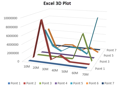
3D Plot in Excel | How to Plot 3D Graphs in Excel?

Multiple data labels (in separate locations on chart) You can do it in a single chart. Create the chart so it has 2 columns of data. At first only the 1 column of data will be displayed. Move that series to the secondary axis. You can now apply different data labels to each series. Attached Files 819208.xlsx‎ (13.8 KB, 264 views) Download Cheers Andy Register To Reply

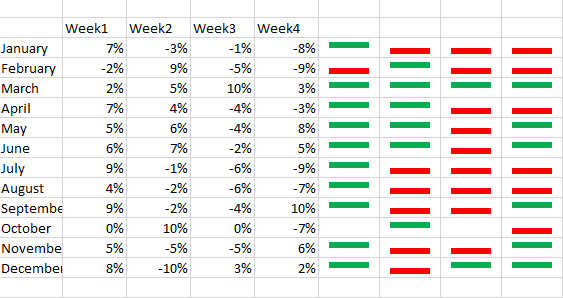
Win Loss Chart in Excel - DataScience Made Simple

Pie of Pie Chart in Excel - Inserting, Customizing, Formatting To add the data labels:- Select the chart and click on + icon at the top right corner of chart. Mark the check box containing data labels. Formatting Data Labels Consequently, this is going to insert default data labels on the chart.

How to Make a Pie Chart in Excel & Add Rich Data Labels to The Chart!

Adding 2nd Data Label Series to Bar of Pie Chart If you use 2 sets of the same data in the chart you can create 2 pie/bar charts, with one appearing on the secondary axis. Make sure the settings for bar/pie formatting are the same. Add data labels to each series. Format one to show names the other values. Within the pie you may want to delete the name data labels. Attached Files

ADMNEXC305308 Excel Training - How to Create a pie chart with data labels - Showezy Excel & Xero ...

Adding data labels to a pie chart - Excel General - OzGrid But it didn't record anything about labels, much less making them bold. In fact, I tried recording multiple macros (create the chart from scratch, modify a created chart, etc.) and still nothing about labels. The macros I recorded without touching the labels look the same as the ones with. Do you know why that is? Thanks a lot.

Data labels on Excel charts « projectwoman.com

How to add axis label to chart in Excel? - ExtendOffice Add axis label to chart in Excel 2013. In Excel 2013, you should do as this: 1. Click to select the chart that you want to insert axis label. 2. Then click the Charts Elements button located the upper-right corner of the chart. In the expanded menu, check Axis Titles option, see screenshot: 3. And both the horizontal and vertical axis text boxes have been added to the chart, then click each of the axis text boxes and enter your own axis labels for X axis and Y axis separately.

How to create doughnut chart in Excel?

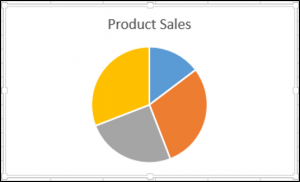
How to Create Pie Charts in Excel (In Easy Steps) Click the + button on the right side of the chart and click the check box next to Data Labels. 10. Click the paintbrush icon on the right side of the chart and change the color scheme of the pie chart. Result: 11. Right click the pie chart and click Format Data Labels. 12. Check Category Name, uncheck Value, check Percentage and click Center.

How to Create and Format a Pie Chart in Excel

How to Make a PIE Chart in Excel (Easy Step-by-Step Guide) Here are the steps to format the data label from the Design tab: Select the chart. This will make the Design tab available in the ribbon. In the Design tab, click on the Add Chart Element (it's in the Chart Layouts group). Hover the cursor on the Data Labels option.

Share :