44 excel donut chart labels

Change the format of data labels in a chart To get there, after adding your data labels, select the data label to format, and then click Chart Elements > Data Labels > More Options. To go to the appropriate area, click one of the four icons ( Fill & Line, Effects, Size & Properties ( Layout & Properties in Outlook or Word), or Label Options) shown here. How to make doughnut chart with outside end labels? - Simple Excel VBA ... In the doughnut type charts Excel gives You no option to change the position of data label. The only setting is to have them inside the chart.

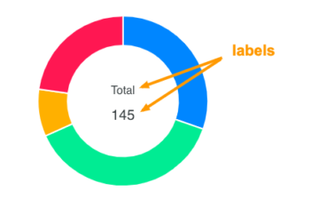
Free Pie Chart Maker - Make Your Own Pie Chart | Visme Create pie charts with our online pie chart maker. Import Excel data or sync to live data with our pie chart maker. Add several data points, data labels to each slice of pie. Chosen by brands large and small. Our pie chart maker is used by over 14,209,854 marketers, communicators, executives and educators from over 120 countries that include: EASY TO EDIT Pie Chart Templates. Make …

Excel donut chart labels

Excel Doughnut chart with leader lines - teylyn Step 1 - doughnut chart with data labels Step 2 -Add the same data series as a pie chart Next, select the data again, categories and values. Copy the data, then click the chart and use the Paste Special command. Specify that the data is a new series and hit OK. You will see the new data series as an outer ring on the doughnut chart. Labels for pie and doughnut charts - Support Center To format labels for pie and doughnut charts: 1. Select your chart or a single slice. Turn the slider on to Show Label. 2. Use the sliders to choose whether to include Name, Value, and Percent. 3. Use the Precision setting allows you to determine how many digits display for numeric values. 4. Gantt project planner - templates.office.com This Gantt chart Excel template makes for a perfect project planner, allowing you to track and synchronize the activities of a project. Based on the long-standing Gantt chart model, this project planning template in Excel uses a simple visual representation to show how a project will be managed over time. You can enter the start dates, duration, and current status of each task and …

Excel donut chart labels. How to make doughnut chart with outside end labels 21 Apr 2020 — Four options to choose: Center to put them in the middle to the piece of your cake. Inside End to place them inside, but just near to the ledge. Doughnut Chart in Excel - GeeksforGeeks Follow the below steps to insert a doughnut chart with single data series: Insert the data in the spreadsheet. We will take the example of data showing the sales of apple between January - August. Select the data (A2:A9, B2:B9). Click on Insert Tab. Select your desired Doughnut chart (Doughnut, Exploded doughnut), under the Other charts. How to create a creative multi-layer Doughnut Chart in Excel By default, all doughnut chart layers have a borderline. As this border line is only disrupting the look, you should remove it for all borders first. After that, select the outer layer of the second (also second biggest) data point and set the fill to No fill. For the third data point we apply the same technique to the two outer layers, and so on. How to Change Excel Chart Data Labels to Custom Values? 05.05.2010 · We all know that Chart Data Labels help us highlight important data points. When you "add data labels" to a chart series, excel can show either "category" , "series" or "data point values" as data labels. But what if you want to have a data label show a different value that one in chart's source data? Use this tip to do that.

How to create doughnut chart in Excel? - ExtendOffice In Excel 2013, click Insert > Insert Pie or Doughnut Chart > Doughnut. See screenshot: 2. Then a doughnut chart is inserted in your worksheet. Now you can right click at all series and select Add Data Labels from the context menu to add the data labels. See screenshots: Now a simple doughnut chart is created. How to Make a Doughnut Chart in Excel | EdrawMax Online Step 1: Select Chart Type. When you open a new drawing page in EdrawMax, go to Insert tab, click Chart or press Ctrl + Alt + R directly to open the Insert Chart window so that you can choose the desired chart type. Here we need to insert a basic doughnut chart into the drawing page, so we can just select " Doughnut Chart " on the window and ... Curved labels in Excel doughnut chart - Microsoft Community All I've seen is that you can display labels in straight lines. You can angle them, rotate them, invert them, but not curve them. You can even make them "dynamic", but no mention of curved text. The simple reality is that in terms of presentation, excel is primitive. . This article shows the label options in 2016, no mention of curves Question: labels in an Excel doughnut chart - Microsoft Tech Community Open your Excel document and click on your chart. In the upper bar you will find the "Diagram Tools". Click on the "Design" tab. In the "Data" group, click the "Select data" button. In the right window you will find the "Horizontal axis label". Click on "Edit". Now enter your desired names or values for the legend.

Pie chart maker | Create a pie graph online - RapidTables.com Use 2 underlines '__' for 1 underline in data labels: 'name__1' will be viewed as 'name_1' Pie chart. Pie chart is circle divided to slices. Each slice represents a numerical value and has slice size proportional to the value. Pie chart types. Circle chart: this is a regular pie chart. 3D pie chart: the chart has 3D look. Excel Charts - Doughnut Chart - Tutorials Point Step 2 − Select the data. Step 3 − On the INSERT tab, in the Charts group, click the Pie chart icon on the Ribbon. It is used to insert a Doughnut chart also. You will see the different types of Doughnut charts available. Step 4 − Point your mouse on the Doughnut icon. A preview of that chart type will be shown on the worksheet. Curve Text in Doughnut chart - Excel Help Forum Re: Curve Text in Doughnut chart. You can link WordArt to a cell using a formula. Just select the shape, click into the formula bar, type = and then select the cell and press Enter. Please remember to mark your thread 'Solved' when appropriate. Progress Doughnut Chart with Conditional Formatting in Excel The entire chart will be shaded with the progress complete color, and we can display the progress percentage in the label to show that it is greater than 100%. Step 2 - Insert the Doughnut Chart With the data range set up, we can now insert the doughnut chart from the Insert tab on the Ribbon. The Doughnut Chart is in the Pie Chart drop-down menu.

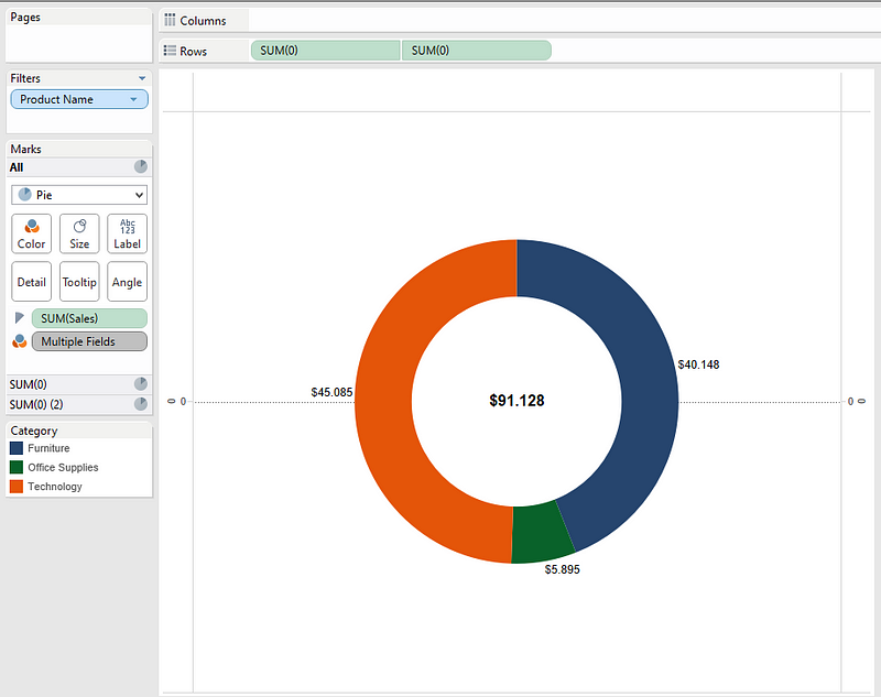
Tableau: Modified pie charts – Leon Agatić – Medium

Excel Doughnut Chart in 3 minutes - Watch Free Excel Video ... - YouTube Doughnut charts is cirular graph which display data in rings, where each ring represents a data series. In Doughnut Chart percentages are displayed in data l...

psd3 - Javascript Pie Chart Library based on d3.js

Create Radial Bar Chart in Excel - Step by step Tutorial Jun 25, 2022 · This unique Excel graph is useful for sales presentations and reports. First, let us see the initial data set! Then, we’ll compare five products. Step 1: Check this range below! You can include the Product Name and Sales fields. The first field is placed in column ‘B’. The second field is in column ‘C’. Using this data set, we’ll ...

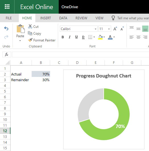
Progress Doughnut Chart with Conditional Formatting in Excel - Excel Campus

Fix label position in doughnut chart? | MrExcel Message Board Turn off data labels. Insert a Text box in to the middle of the donut, select the edge of the text box and in the formula bar hit = then select the cell that contains the progress figure. You can format this to however you want it, it will update and it won't move. Click to expand... Oh wow! I always thought text-boxes were just text-boxes.

Pie Chart Templates

How to add leader lines to doughnut chart in Excel? Select data and click Insert > Other Charts > Doughnut. In Excel 2013, click Insert > Insert Pie or Doughnut Chart > Doughnut. 2. Select your original data again, and copy it by pressing Ctrl + C simultaneously, and then click at the inserted doughnut chart, then go to click Home > Paste > Paste Special. See screenshot: 3.

Pie / Donut Chart Guide & Documentation – ApexCharts.js

excel - Positioning labels on a donut-chart - Stack Overflow The option to place the labels outside the chart is not available on the doughnut chart options: like they do on a pie chart: However, you could perform a trick using a pie chart and a white circle to make it look like a doughnut by doing the following: Sub AddCircle () 'Get chart size and position: Dim CH01 As Chart: Set CH01 = ThisWorkbook ...

Share :