44 labels in excel 2010

Excel 2010 Pivot Tables Multiple Worksheets Excel 2010 pivot tables multiple worksheets. Creating a Pivot Table with Multiple Sheets Alt D is the access key for MS Excel and after that by pressing P after that well enter to the Pivot table and Pivot Chart Wizard. Start Your Free Two Week Trial Today. Click the button to open the PivotTable and PivotChart Wizard. Two-Level Axis Labels (Microsoft Excel) Excel automatically recognizes that you have two rows being used for the X-axis labels, and formats the chart correctly. Since the X-axis labels appear beneath the chart data, the order of the label rows is reversed—exactly as mentioned at the first of this tip. (See Figure 1.) Figure 1. Two-level axis labels are created automatically by Excel.

How to Add Labels to Scatterplot Points in Excel - Statology Step 3: Add Labels to Points Next, click anywhere on the chart until a green plus (+) sign appears in the top right corner. Then click Data Labels, then click More Options… In the Format Data Labels window that appears on the right of the screen, uncheck the box next to Y Value and check the box next to Value From Cells.

Labels in excel 2010

How to calculate variance in Excel? | Microsoft Excel Tips | Excel ... Labels in first row - there are no labels in my data table Output Range - choose where you want to get your variance calculated (I chose the same Sheet $G$1:$T$18) Summary statistics - make sure it is checked And this is how to see my Statistics summary. Sample variance is calculated in row 8. Template You can download the Template here - Download Manage sensitivity labels in Office apps - Microsoft Purview ... Set Use the Sensitivity feature in Office to apply and view sensitivity labels to 0. If you later need to revert this configuration, change the value to 1. You might also need to change this value to 1 if the Sensitivity button isn't displayed on the ribbon as expected. For example, a previous administrator turned this labeling setting off. Pivot Table data range in Excel - Microsoft Community After the data is loaded to Excel, in form of Excel Tables on a worksheet, the data can be manipulated in the table, or fed into a PivoTable and then to a PivotChart. PowerQuery allows you to use a "Click and Drag" user interface from the Ribbon and right click context menus to generate the required code in the background.

Labels in excel 2010. excel - VBA Collection (Array?) of Controls - Stack Overflow But you need to work column wise in your loops. So first the column loop and inside the rows loop. With a Select Case you can switch for your columns from labels to comboboxes to textboxes. So in your case you still have 5 columns with each 10 controls but the first column is labels and the last column is comboboxes: How to Get Rows to Repeat at Top - Excel 2010 - Solve Your Tech How to Repeat Rows in Excel 2010 Click the Page Layout tab. Click the Page Setup dialog launcher or the Print Titles button. Click the Sheet tab at the top of the Page Setup window. Click inside the Rows to repeat at top field. Click the number of the row that you want to repeat, or manually enter the $X:$X data. Click the OK button. Advanced Microsoft Excel 2010 | University of Louisiana at Lafayette Advanced capabilities in Microsoft Excel 2010 allow you to better consolidate, analyze, and report on data. This course provides expert instruction and hands-on exercises to help you master analysis tools, PivotTables, conditional formatting, and other advanced features. How to Print Labels from Excel - Lifewire Choose Start Mail Merge > Labels . Choose the brand in the Label Vendors box and then choose the product number, which is listed on the label package. You can also select New Label if you want to enter custom label dimensions. Click OK when you are ready to proceed. Connect the Worksheet to the Labels

support.microsoft.com › en-us › officeCreate and print mailing labels for an address list in Excel Create and print mailing labels for an address list in Excel. Column names in your spreadsheet match the field names you want to insert in your labels. All data to be merged is present in the first sheet of your spreadsheet. Postal code data is correctly formatted in the spreadsheet so that Word can ... Sorting the 5th column in a pivot - excelforum.com Include a BEFORE sheet and an AFTER sheet in the workbook if needed to show the process you're trying to complete or automate. Make sure your desired results are shown, mock them up manually if necessary. Remember to desensitize the data. Click on GO ADVANCED and then scroll down to Manage Attachments to open the upload window. How to Create a Mekko Chart (Marimekko) in Excel - Quick Guide Here are the steps to create a Mekko chart: #1: Set up a helper table and add data. #2: Append the helper table with zeros. #3: Apply a custom number format. #4: Calculate and add segment values. #5: Set up the horizontal axis values. #6: Calculate midpoints. #7: Add labels for rows and columns. How Do I Create A Macro In Excel 2010 .pdf - 50.iucnredlist Use the \label macro, as usual to label a line. When you use \ref to reference the line, the \ref will be subtitued with the corresponding line number. When using the algorithmicx package togedher with the algorithm package, then you can label both the algorithm and the line, and use the \algref macro to reference a given line from a given ...

Pivot table from Power BI data in Excel 2013 According to this article, the prereq for this feature is Excel 2010 SP1, so it should work in Excel 2013. Has anybody run into this issue when trying to access Power BI data in Excel 2013? Thanks, Matt. Solved! Go to Solution. Labels: Labels: Need Help; Message 1 of 3 107 Views 0 Reply. 1 ACCEPTED SOLUTION GilbertQ. Super User Mark as New ... Fill Blank Cells in Excel Column - Contextures Excel Tips 1) Select Empty Cells. The first main step is to select all the blank cells that you want to fill. To select the empty cells with Excel's built in Go To Special feature, follow these steps: Select columns A and B, that contain the blank cells. Use the Ribbon commands: On the Excel Ribbon's Home tab, in the Editing group, click Find & Select. Sequentially Numbered Labels - Microsoft Word Tips In the top-left label, type the word Exhibit, followed by a space. Press Ctrl+F9. Word inserts a pair of field braces in the label. Type SEQ and a space. Type a name for this sequence of numbers, such as "exhibit" (without the quote marks). Press F9. The field is collapsed and a number appears in your label. How To Add Data Labels In Excel | Nabludatel Click any data label to select all data labels, and then click the specified data label to. Press The Ok Button To Close The Change Chart Type Dialog Box. A menu of data label placement options appears: Select each item where you want the custom label one at a time. Finally, repeat for all your chart laebls.

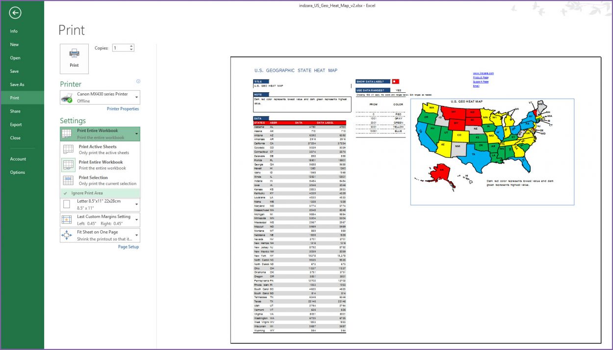
U.S. GEOGRAPHIC STATE HEAT MAP - EXCEL TEMPLATE

answers.microsoft.com › en-us › msofficeHow to create column labels in Excel 2010 - Microsoft Community Jul 16, 2012 · In row1 enter Label1 in A1, Lable2 in B1 and so on till the column you have data which you want in your table. Once this works then you can replace Lable1 etc by the true labels you want... this will tell you which lable is creating a problem. If this response answers your question then please mark as Answer. It helps others who browse.

Nokia C7 Specification Review ,Price,Features,| Nokia Smartphones 2010 | New Gadget Handphone Laptop

Excel 2010 Pivot Chart Axis label - community.spiceworks.com Excel 2010 Pivot Chart Axis label Posted by DLB. Microsoft Office. I have the horizontal axis configured with 2 fields (date and time), but I can't figure out how to format the date text so that it doesn't run together. See attachment.

Share :