45 how to add different data labels in excel
How to add Data bar in a diffferent cell that already has different ... Once your problem is solved, reply to the answer (s) saying Solution Verified to close the thread. Follow the submission rules -- particularly 1 and 2. To fix the body, click edit. To fix your title, delete and re-post. Include your Excel version and all other relevant information. Failing to follow these steps may result in your post being ... How To Create Labels In Excel - newall.northminster.info The create cards dialog window will appear: Add data labels to a scatter plot chart. Source: . Add data labels to a chart. However, this causes the labels to overlap in some areas and makes it difficult to read. Source: ambitiousmares.blogspot.com. Click axis titles to put a checkmark in the axis title checkbox.
Overview of data types in Excel add-ins - Office Add-ins Custom functions accept data types as both inputs to custom functions and outputs of custom functions, and custom functions use the same JSON schema for data types as the Excel JavaScript API. This data types JSON schema is maintained as custom functions calculate and evaluate. To learn more about integrating data types with your custom ...

How to add different data labels in excel
Error bars in Excel: standard and custom - Ablebits.com 25 comments . Christian Appiah says: June 21, 2022 at 10:22 am 1 I am developing a STAKEHOLDER MAPPING chart. I need the names of the stakeholders to be listed in the 4 quadrants of the chart according to their respective scores. How to add trendline in Excel chart - Ablebits.com Draw different trendline types for the same data series. To make two or more different trendlines for the same data series, add the first trendline as usual, and then do one of the following: Right-click the data series, select Add Trendline… in the context menu, and then choose a different trend line type on the pane. How to Create a Map in Excel (2 Easy Methods) - ExcelDemy First, select the range of cells B4 to C11. Then, go to the Insert tab in the ribbon. From the Charts group, select Maps. Next, select the Filled Map from the drop-down list of Maps. As a result, it will provide us following map chart of countries. Then, click the plus (+) sign beside the map chart.
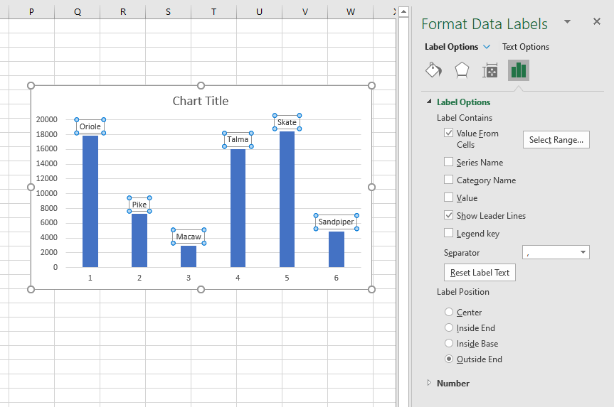
How to add different data labels in excel. How to Display Percentage in an Excel Graph (3 Methods) Display Percentage in Graph. Select the Helper columns and click on the plus icon. Then go to the More Options via the right arrow beside the Data Labels. Select Chart on the Format Data Labels dialog box. Uncheck the Value option. Check the Value From Cells option. Data validation in Excel: how to add, use and remove - Ablebits.com Method 1: Regular way to remove data validation. Normally, to remove data validation in Excel worksheets, you proceed with these steps: Select the cell (s) with data validation. On the Data tab, click the Data Validation button. On the Settings tab, click the Clear All button, and then click OK. Labeling in the Microsoft Purview Data Map - Microsoft Purview Labeling for SQL databases. In addition to labeling for schematized data assets, the Microsoft Purview Data Map also supports labeling for SQL database columns using the SQL data classification in SQL Server Management Studio (SSMS).While Microsoft Purview uses the global sensitivity labels, SSMS only uses labels defined locally.. Labeling in Microsoft Purview and labeling in SSMS are separate ... Manage sensitivity labels in Office apps - Microsoft Purview ... Set Use the Sensitivity feature in Office to apply and view sensitivity labels to 0. If you later need to revert this configuration, change the value to 1. You might also need to change this value to 1 if the Sensitivity button isn't displayed on the ribbon as expected.
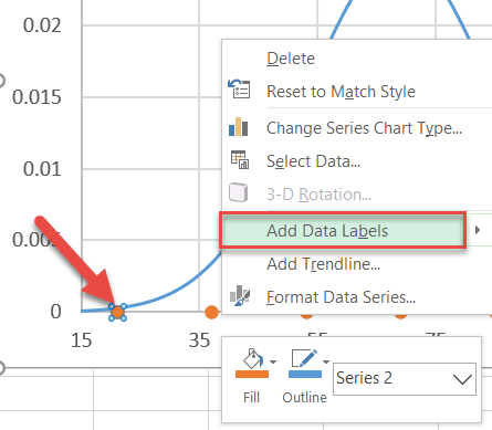
Add data labels to column or bar chart in R - Data Cornering If you are using the ggplot2 package, then there are two options to add data labels to columns in the chart. The first of those two is by using geom_text. If your columns are vertical, use the vjust argument to put them above or below the tops of the bars. Here is an example with the data labels above the bars. How to make a pie chart in Excel - Ablebits.com Adding data labels to Excel pie charts. In this pie chart example, we are going to add labels to all data points. To do this, click the Chart Elements button in the upper-right corner of your pie graph, and select the Data Labels option. Additionally, you may want to change the Excel pie chart labels location by clicking the arrow next to Data ... Find, label and highlight a certain data point in Excel scatter graph Here's how: Click on the highlighted data point to select it. Click the Chart Elements button. Select the Data Labels box and choose where to position the label. By default, Excel shows one numeric value for the label, y value in our case. To display both x and y values, right-click the label, click Format Data Labels…, select the X Value and ... How to add a line in Excel graph: average line, benchmark, etc. Right-click the selected data point and pick Add Data Label in the context menu: The label will appear at the end of the line giving more information to your chart viewers: Add a text label for the line. To improve your graph further, you may wish to add a text label to the line to indicate what it actually is. Here are the steps for this set up:
How to Create Mailing Labels in Excel - Sheetaki In the Mailings tab, click on the option Start Mail Merge. In the Label Options dialog box, select the type of label format you want to use. In this example, we'll select the option with the product number '30 Per Page'. Click on OK to apply the label format to the current document. How to Add Secondary Axis in Excel (3 Useful Methods) - ExcelDemy Steps: Firstly, right-click on any of the bars of the chart > go to Format Data Series. Secondly, in the Format Data Series window, select Secondary Axis. Now, click the chart > select the icon of Chart Elements > click the Axes icon > select Secondary Horizontal. We'll see that a secondary X axis is added like this. How to mail merge and print labels from Excel to Word - Ablebits.com Select document type. The Mail Merge pane will open in the right part of the screen. In the first step of the wizard, you select Labels and click Next: Starting document near the bottom. (Or you can go to the Mailings tab > Start Mail Merge group and click Start Mail Merge > Labels .) Choose the starting document. Learn about sensitivity labels - Microsoft Purview (compliance) In all these cases, sensitivity labels from Microsoft Purview can help you take the right actions on the right content. With sensitivity labels, you can classify data across your organization, and enforce protection settings based on that classification. That protection then stays with the content. For more information about these and other ...

Directly Labeling Excel Charts - PolicyViz
I can't arrange my labels on my x axis in PowerBI correctly? : r/excel Blue. Red. Green. In my data table, I have the levels of each color in a separate column, so all Orange shows as 1, all Blue as 2, all Red as 3, and all Green as 4. When I add color_name to my column chart in the x axis, it sorts alphabetically. When I add color_level to the x axis, it sorts correctly but displays the number of each level, not ...

Quick Tip: Excel 2013 offers flexible data labels | TechRepublic
Excel Charts Adding Labels To An Xy Scatter Chart Youtube How to create an x y scatter chart with data label- there isn39t a function to do it explicitly in excel but it can be done with a macro- the microsoft kno- Exc. Home; News; Technology. All; Coding; Hosting; Create Device Mockups in Browser with DeviceMock. Creating A Local Server From A Public Address.
How to add data labels from different column in an Excel chart?
How to Create a Map in Excel (2 Easy Methods) - ExcelDemy First, select the range of cells B4 to C11. Then, go to the Insert tab in the ribbon. From the Charts group, select Maps. Next, select the Filled Map from the drop-down list of Maps. As a result, it will provide us following map chart of countries. Then, click the plus (+) sign beside the map chart.

How to Add Data Labels to an Excel 2010 Chart - dummies
How to add trendline in Excel chart - Ablebits.com Draw different trendline types for the same data series. To make two or more different trendlines for the same data series, add the first trendline as usual, and then do one of the following: Right-click the data series, select Add Trendline… in the context menu, and then choose a different trend line type on the pane.
How to Add Data Labels to a Chart - ExcelNotes
Error bars in Excel: standard and custom - Ablebits.com 25 comments . Christian Appiah says: June 21, 2022 at 10:22 am 1 I am developing a STAKEHOLDER MAPPING chart. I need the names of the stakeholders to be listed in the 4 quadrants of the chart according to their respective scores.
/Capture-e92aa05671d543ceaf94080eb2687619.JPG)
Understanding Excel Chart Data Series, Data Points, and Data ...
Directly Labeling Excel Charts - PolicyViz

How to Change Excel Chart Data Labels to Custom Values?

How to Use Cell Values for Excel Chart Labels

how to add data labels into Excel graphs — storytelling with data

Format Data Labels in Excel- Instructions - TeachUcomp, Inc.

How to Add Data Labels to your Excel Chart in Excel 2013
Using the CONCAT function to create custom data labels for an ...
Add / Move Data Labels in Charts – Excel & Google Sheets ...

How to add or move data labels in Excel chart?

Enable or Disable Excel Data Labels at the click of a button ...

424 How to add data label to line chart in Excel 2016

Custom Chart Data Labels In Excel With Formulas
Excel macro to fix overlapping data labels in line chart ...
how to add data labels into Excel graphs — storytelling with data

Custom Data Labels with Colors and Symbols in Excel Charts ...

Custom Data Labels with Colors and Symbols in Excel Charts ...
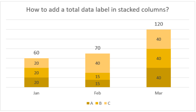
Add Data Labels for Total to Stacked Columns in #Excel | wmfexcel

Add or remove data labels in a chart

Custom data labels in a chart

How to add total labels to stacked column chart in Excel?

Using the CONCAT function to create custom data labels for an ...

Apply Custom Data Labels to Charted Points - Peltier Tech

Microsoft Excel Tutorials: Add Data Labels to a Pie Chart

How do I add Data Labels for multiple Low Points Only! : r/excel

Google Workspace Updates: Get more control over chart data ...

Google Workspace Updates: New chart text and number ...

How to Add Axis Labels to a Chart in Excel | CustomGuide

How-to Use Data Labels from a Range in an Excel Chart - Excel ...

How to Add Data Labels in Excel - Excelchat | Excelchat

How-to Use Data Labels from a Range in an Excel Chart - Excel ...
insert-the-default-data-labels - Automate Excel

Adding rich data labels to charts in Excel 2013 | Microsoft ...

Stagger long axis labels and make one label stand out in an ...
Custom data labels in a chart
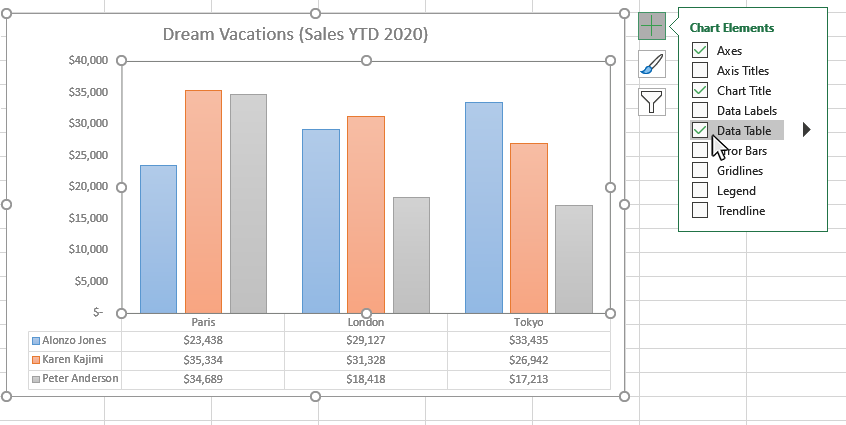
How to Add Data Tables to a Chart in Excel - Business ...

Change the format of data labels in a chart

Add Custom Labels to x-y Scatter plot in Excel - DataScience ...

Apply Custom Data Labels to Charted Points - Peltier Tech

How to add or move data labels in Excel chart?
Post a Comment for "45 how to add different data labels in excel"